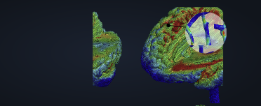
You cannot put a strain gauge inside a living brain. So how does anyone know how much the tissue stretched during a tackle? The answer is that they don’t measure it — they simulate it, using a digital reconstruction of the head called a finite-element (FE) model.
This article is a short tour of those models: what they are, why they’re trusted, and why — despite being trusted — they’re too slow to use on their own. That last point is the whole reason trace* exists.
Breaking the head into tiny pieces
“Finite element” is a method engineers use to work out how a complicated object deforms under load. The trick is to chop the object into a very large number of tiny, simple shapes — usually tetrahedra, the 3D equivalent of triangles — and solve the physics for each little piece, accounting for how it pushes and pulls on its neighbours.
A finite-element head model does exactly this for the anatomy inside the skull:
- the skull and scalp,
- the brain itself, split into grey and white matter,
- the cerebrospinal fluid that the brain floats in,
- the ventricles and the membranes (the falx and tentorium) that partition the brain.
Each tissue is given its own mechanical properties — how stiff it is, how it behaves when loaded quickly versus slowly, how it resists being sheared. The Imperial College model that trace* is built around represents roughly a million elements across about a dozen tissues (Ghajari et al., 2017).
What you put in, and what you get out
The input is the head kinematics — the same accelerations and rotations an instrumented mouthguard records. You apply that motion to the skull, and a solver computes, millisecond by millisecond, how every one of those million elements deforms.
The output is a complete map of strain throughout the brain: how much each region stretched, when, and in which direction. From that map you can read off the figures the rest of trace* talks about — the per-region maximum principal strain, and the 90th-percentile summary (MPS90) used to avoid being thrown off by a single noisy element.
Why we trust these simulations
A model is only useful if its predictions match reality. FE brain models are validated in two main ways:
- Against cadaver experiments. Classic studies implanted markers in donated heads, struck them under controlled conditions, and filmed how the brain moved with high-speed X-ray. A good model, given the same input, should reproduce that motion. The Imperial and KTH models are both anchored to this kind of data.
- Against real pathology. The striking result behind the Imperial model is that the regions it predicts to experience the highest strain line up with where chronic traumatic encephalopathy pathology is actually found at post-mortem — at the depths of the cortical folds, around blood vessels (Ghajari et al., 2017). More recent work goes further and links simulated strain patterns to where axonal injury is seen (Donat et al., 2021).
That convergence — physics on one side, biology on the other — is why these models are treated as a ground truth for brain deformation, and why newer studies use them to compare protected versus unprotected impacts in sport (Hodges et al., 2025).
The catch: they are painfully slow
All this realism has a price. Running a single high-resolution impact through a model like this takes five to six hours on a high-performance computing cluster. That’s fine for a research study analysing a few dozen carefully chosen impacts. It is hopeless for a pitch-side tablet that needs an answer before the next lineout.
You also can’t run one on a phone, and you certainly can’t run one for every one of the thousands of impacts an athlete absorbs across a season.
Where trace* comes in
This is the gap trace* fills. Instead of running the simulation live, it learns from the simulation’s output: thousands of impacts that have already been put through the FE model, each paired with the strain map it produced. A fast machine-learning model is then trained to predict that strain map directly from the mouthguard kinematics — in milliseconds rather than hours (Chan et al., 2025).
You give up a little accuracy compared with the full simulation. In return you can do it everywhere, for every impact, in real time. The slow, careful model is the teacher; trace* is the fast student that learned its answers.
Sources & further reading
- Ghajari, M., Hellyer, P. & Sharp, D. (2017) — Computational modelling of traumatic brain injury predicts the location of chronic traumatic encephalopathy pathology. Brain 140 (2). — The Imperial College brain model, validated against the location of CTE pathology.
- Donat, C. K. et al. (2021) — From biomechanics to pathology: predicting axonal injury from patterns of strain after traumatic brain injury. Brain 144 (1). — Links simulated strain to where axonal damage is actually seen.
- Hajiaghamemar, M. et al. (2021) — Multi-scale white matter tract embedded brain finite element model. Biomechanics and Modeling in Mechanobiology 20.
- Hodges, C. et al. (2025) — Computational modelling of protected and unprotected head impacts in sport.
- Chan, E. Y. K., Yu, X., Qin, C. & Ghajari, M. (2025) — Balancing efficiency and accuracy. Engineering Applications of Artificial Intelligence 162, 112489.